Final Project: Mining Process with Real World Ski Resort Data Set
Project Goal
The ski resort data set is collected from real world and we can expect it would contain noise and anomalies due to the various variances and errors in the data collection process. The goal of the project to explore the data set methodically, distinguish the noise data with data-preprocessing process, and discover the internal data pattern with by using a proper mining strategy. The entire mining process and data anaylze result is helpful to understand and characterize the pattern inside the dataset.
Ski Resort Data Set
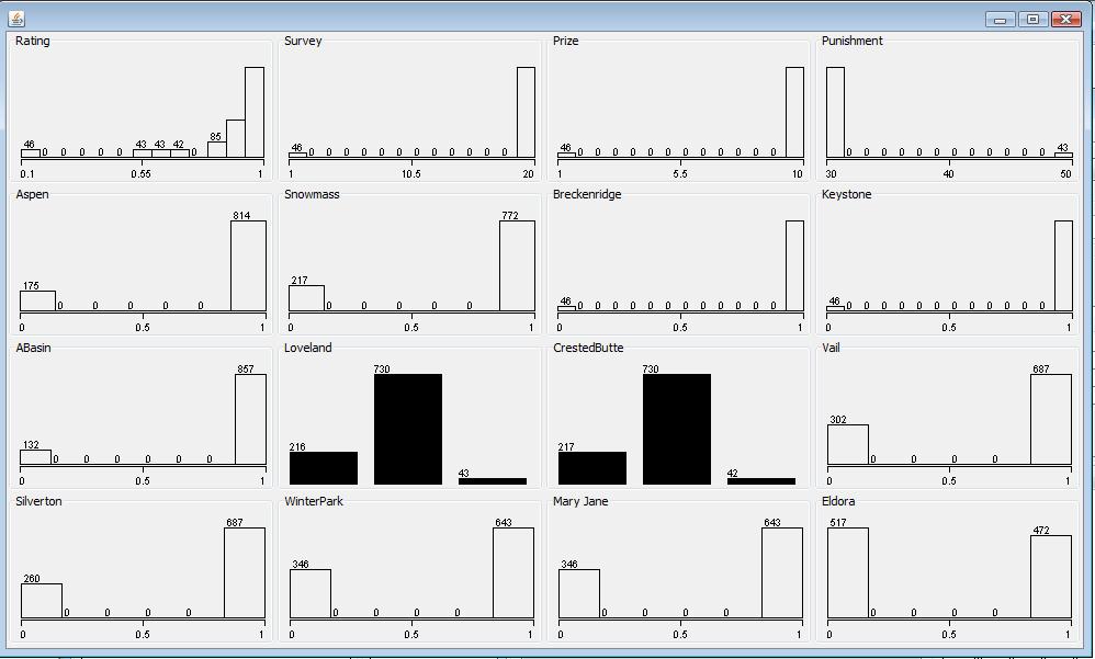
The Ski Resort Data Set is given from Data Mining Course by Yong Bakos. It is a raw data file in .csv format. I use weka to load the data file and save the dataset as final.arff file in default ARFF file format for future processing. It contains 989 data objects and each object has 16 attributes. The data schema is shown as below. All the data attribute are numeric or nomial. The attribute set rating, Survey, Prize, Punishment represents the overall assessment from a subject. The other attribute set Aspen, Snowmass, ..., Eldora represents the different ski resorts a subject rates.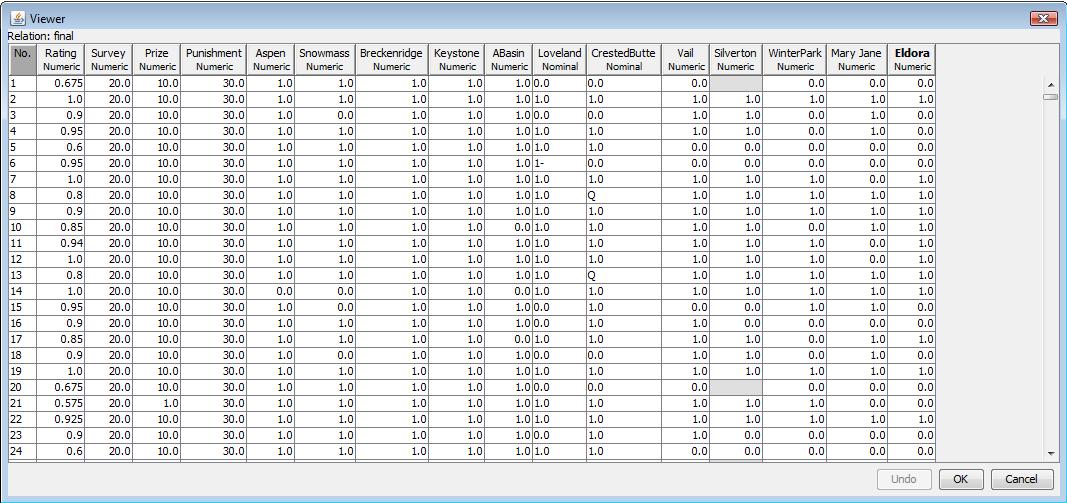 The visualization plot of the attribute sets is as below. Four attributes are numeric, 10 attributes are binary attributes, and two attributes are nominal.
Data Mining Toolkit
The following data mining algorithms and tasks are performed in WEKA3.6. WEKA is open source software. It contains tools for data pre-processing, classification, regression, clustering, association rules, and visualization. WEKA 3.6 is the latest stable version of WEKA. I installed WEKA 3.6 on Windows XP with JDK 1.6.Data Pre-Processing
I first looked at the data objects with missing values and removed the incomplete data from the dataset. Then I used Density-Based cluster algorithm to detect whether there are anomalies in the data set. If the cluster algorithm found anomal data points far from the most data points, the anomal data points are probably noise data and will be removed from data set as well.
Remove Instances Containing Missing Value
The explore tool in WEKA shows excellent statistic result for each data attribute, including the min, max, mean, standard deviation, the number of distinct value and whether there is missing value in the data set. It is straightforward to find out that Loveland and Crested Butte attributes have confused values in certain data objects. Since Loveland and CrestedButte represent the selected ski resort, we can infer that they should be binary attribute as other ski resort attribute set. Thus the value "1-" and "Q" are highly possible error data objects and should be removed from data set. And Silverton attribute has 4% missing values of the whole data set, which are 42 data records. I decided to remove theses instance containning missing value as well because we do not have any prior knowledge about the incomplete data record.
- Unclear "1-" value in Loveland Attribute
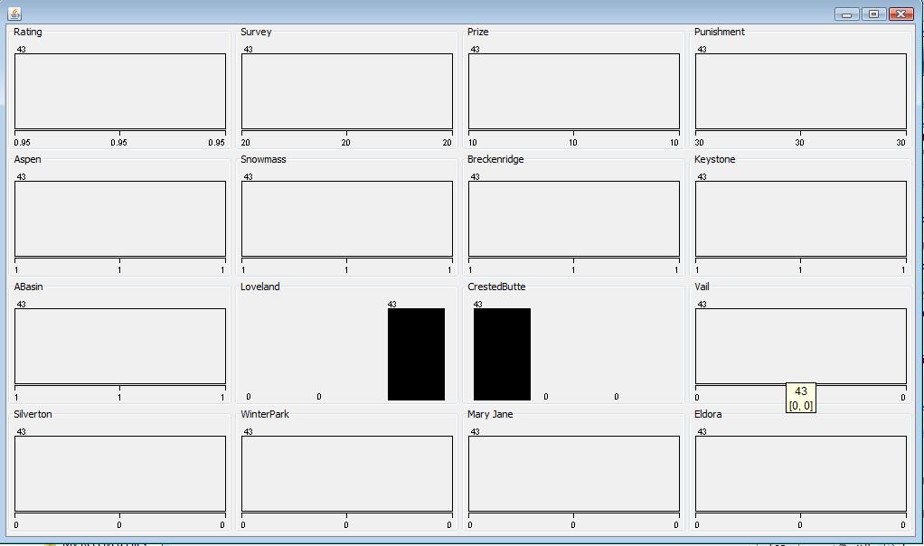
To analyze the data objects containing "1-" value in Loveland attribute, I used a filter filters.unsupervised.instance.SubsetByExpression to select the subset of "1-" data objects. 43 data objects contains "1-" value and they have the same value in all the attributes. The visualized plot of the "1-" subset data shows that they have same distribution. The consistent "1-" data records are more likely introduced by particular error. Thus it is reasonable to remove the 43 "1-" subset data from the data set.
- Unclear "Q" value in CrestedButte Attribute
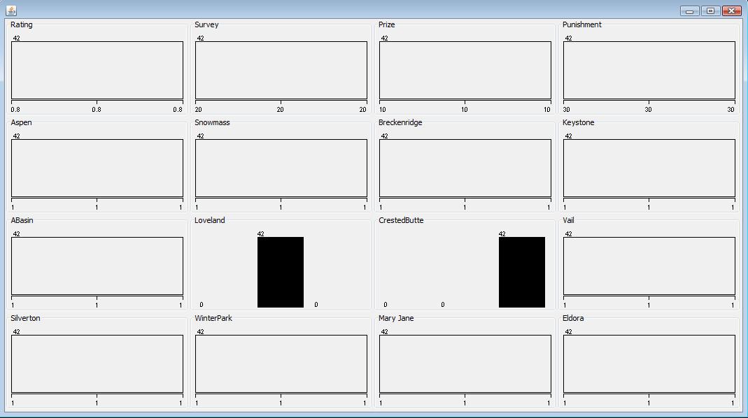
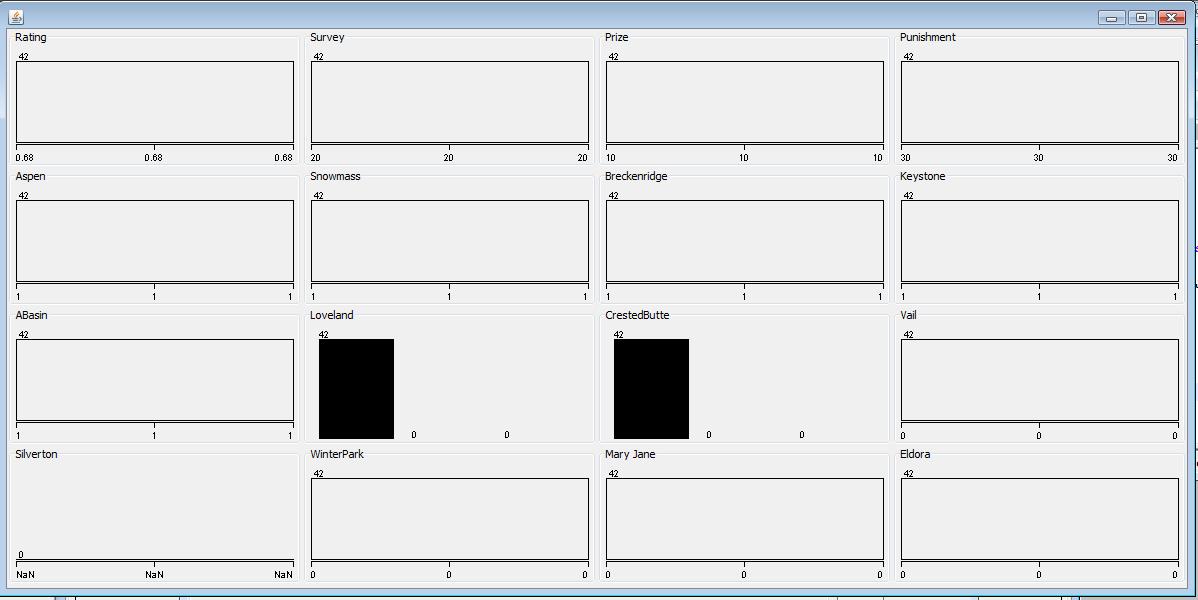
I used the same filter to identify the subset of "Q" data object with different filter parameters ATT10 is 'Q'. Here ATT10 represents the CrestedButte Attribute. After applied the filter in the data set, it filters out the all the "Q" subset data. The subset has 42 data objects. Similarly, all the data objects have the same value in all the attributes, as shown in the following visulized plot of "Q" data subset. Due to the same reason, I removed the 42 "Q" subset data from data set as well.
- Missing value "?" in Silverton Attribute
The same filter is used again to filter out the subset containing missing value "?" in Silver Attribute. The "?" subset contains 42 data objects and all of them have same value in all the attributes, shown in the following plot. Then I removed the "?" subset data from the data set as well.
After removing all the unclear and missing values in the dataset, I saved the processed data set in WEKA explore as final-remove-missing.arff for the data analyze and processing in next step.
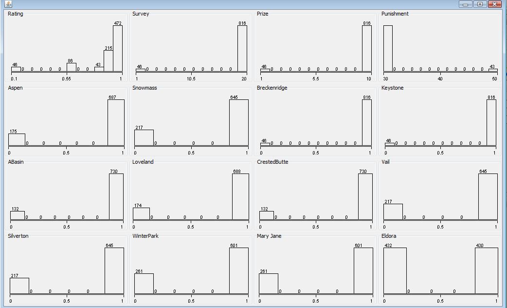
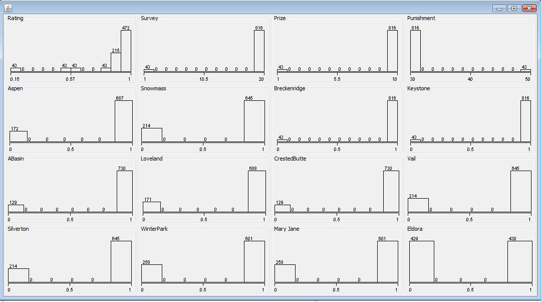
Loading the processed data set file final-remove-missing.arff, it shows all the valid data objects. It contains 862 data objects without unclear or missing values. Taking out "1-" value from Loveland attribute and "Q" value from CrestedButte attribute, they are binary attributes which is same as other ski resort attribute sets.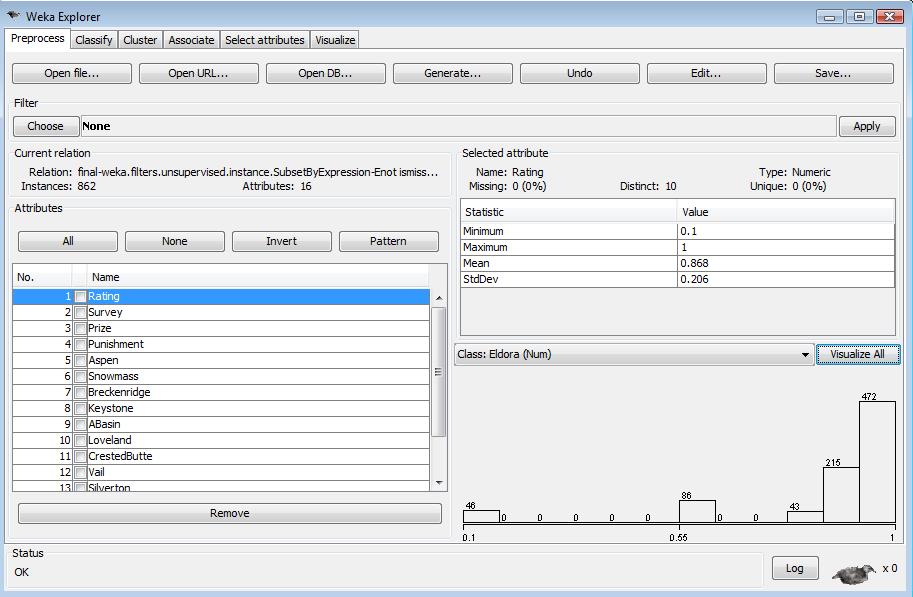
The visualize plot of processed data set is as below.
Detect Anomalies
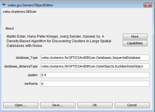
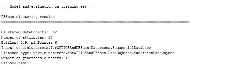
Next, I applied the DBscan cluster algorithm in the data set to make inital data analyze. The DBSCAN algorithm clusteres the data points based on the density. Since I do not have prior knowledge about the noise data and valid data pattern in ski resort dataset, it is unlikely that noise data can be identified by the supervised classification method. The DBSCAN algorithm is an intuitive strategy to group the data points and find out the anomaliers which are far from the normal data points. Following is the configuration page for DBSCAN algorithms.
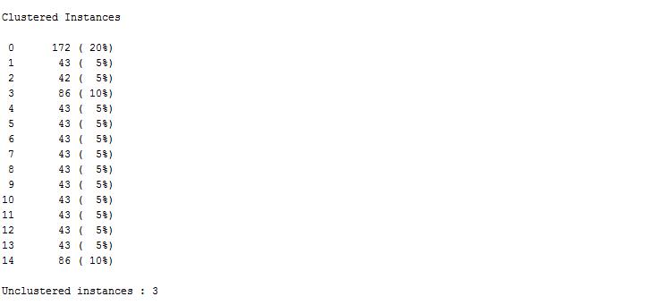
DBSCAN algorithm finishes the clustering process in a short time. It groups the data set into 15 groups. However, there are 3 data points which are failed to be clustered. The unclustered instances are far from the other normal data points and thus can not be grouped in the processes. Those 3 unclustered instances are identified as anomalier.
 After looking through the cluster results for the normal data points, it can be found that 3 unclustered data points having rate value 0.1.
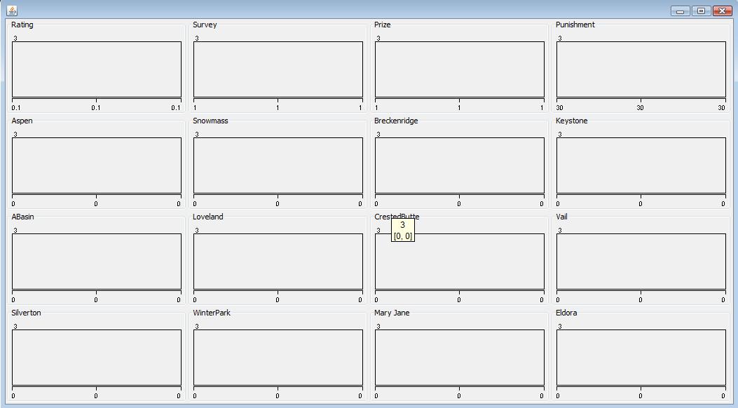
Here is the visualize plot for 3 noise data instances.All of them have 0 value in binary ski resort attributes which seems that non ski resorts are selected in the survey. If so, these 3 data records do not contribute the data processing. Also the rating and survey value is also far from the rest data points and unreasonably low.
After looking through the cluster results for the normal data points, it can be found that 3 unclustered data points having rate value 0.1.
Here is the visualize plot for 3 noise data instances.All of them have 0 value in binary ski resort attributes which seems that non ski resorts are selected in the survey. If so, these 3 data records do not contribute the data processing. Also the rating and survey value is also far from the rest data points and unreasonably low.
 Similarly, the 3 noise data points are removed from data set by using SubsetByExpression filter. The processed data set is saved as final-remove-noise.arff. Now it contains 859 data points and the visualized plot is shown as below.
Mining Processes
In the mining process, I applied four different strategies to analyze the internal pattern of the data set. Simple Kmens distinguish the data set into well seperated groups. NaiveBayes and Decision Tree classifiers finds out the group characteristic of each different class. At last, I used association algorithm to figure out the potential correlation relationship among selected attribute sets.
Simple KMeans Clustering Analyze
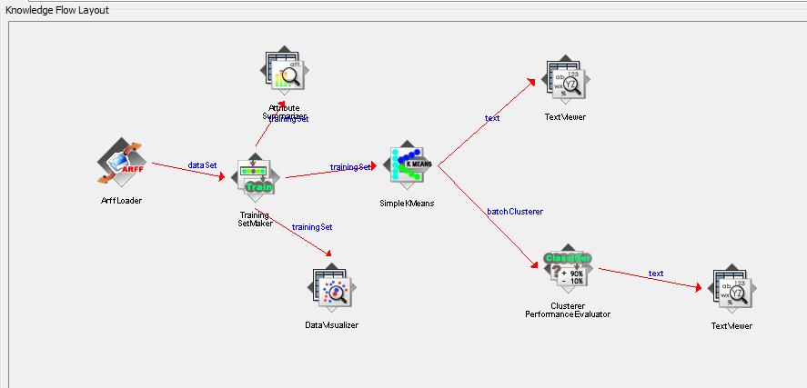
The KMeans algorithm is an effective and simple algorithm to analyse the group characterize of the data set. Followins is the workflow I created with SimpleKMeans algorithm in WEKA. Since the data set has been pre-processed in WEKA explor tool. Here I just used ArffLoader to load the processed data set file final-remove-noise.arff, and then created training data set which is processed with SimpleKMeans module. The other modules in the workflow is tool to view the result of data process results. The WEKA project file is here.
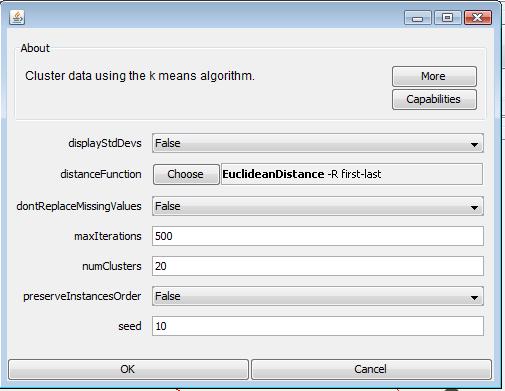
KMeans requires a parameter of number of clusters. Defining a proper number of clusters is important to get accurate analyse result. I tried to group the data set with different number of clusters: 5, 15, 20, 25 and found that using 20 as parameter shows the best result in terms of sum of squared error. If using less than 20 as paramters, the sum of squared error grows significiantly which means inacuurate cluster results. If using larger than 20 as parameters, Kmeans algorithm ends up with 20 clusters as well. The experiments shows that 20 clusters are the optimal clusters for KMeans algorithm in this dataset.
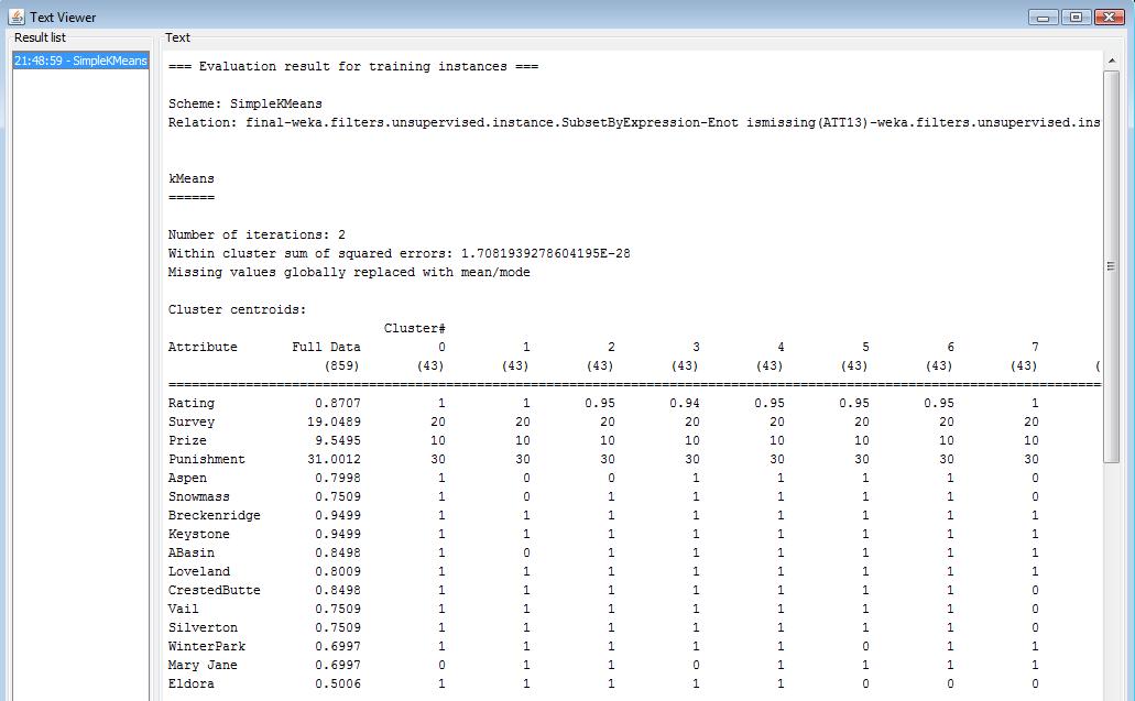
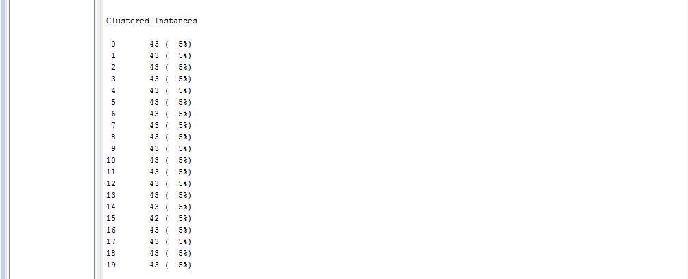
Here is the cluster results with K-means algorithm. The data points are well grouped into 20 clusters. Each cluster includes 5% data points. And the sum of squared error is almost 0. More text detail can be viewed here.
Naive Bayesian Classifier Analyse
The Naive Bayesian classifier is a practical strategy to classify the data objects when the relationship between attributes and selected class lable is not deterministic. Followins is the workflow I created with Naive Bayesian algorithm in WEKA. Since Naive Bayessian classifier requires the attributes are nominal class type, I first used NumbericToNominal Filter to transform the numberic attributes into nominal attributes. Then I discretize the ranking attributes into 5 class lables by using MergeTwoValues Filter. Also Naive Bayesian classifer needs we select a class lable for prediction. I used ranking attribute since other attributes only have two class lables and do not have much groups to be classified. The WEKA project file is here.
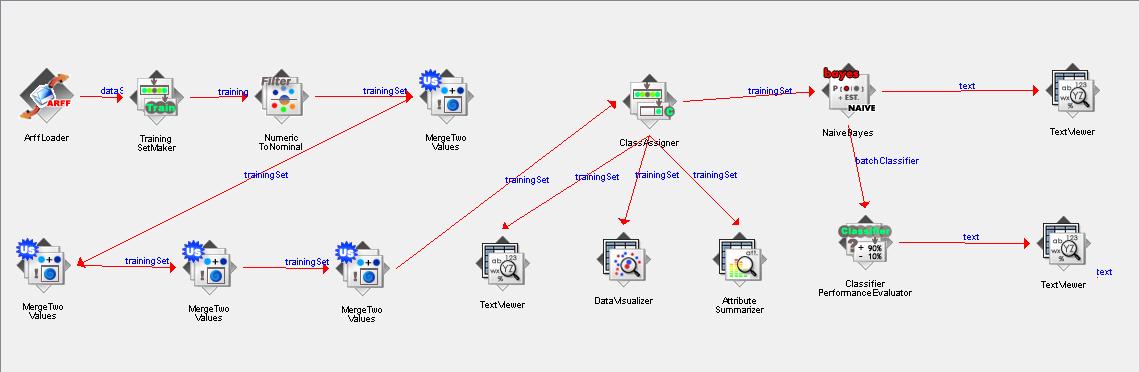
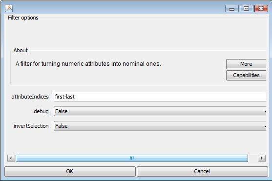
The NumbericToNominal Filter assignes a nominal class lable to each distinct numeric value. With the following configuration, we replace the numberic value with its corresponding nominal class lable for all the attributes. Most attributes are binary attributes, and then they are replaced as two class lable 0 and 1 after transformation. The rating attribute has 9 distinct values, thus it is transformed as a class object with 9 values as well.
The NumbericToNominal Filter is appropriate to discretize the binary attribute into two class lable. However, rating attribute has 9 distinct values. If we have each distinct values as a nominal class lable, then we might fail to aggregate the records from different distinct values and degrade the accuracy of classifier. I tried different strategies to discretize the rating value with proper interval in order to minimize the classification error in terms of Kappa statistic metric. The data sample are scattered from 0.15 to 0.85, and tends to be groups when rating value is greater 0.9. Based on the data characteris and experiments with NaiveBayes Classifer, I mergered all the rating value greater than 0.9 into one class lable. In the workflow, I iteratively used MergeTwoValues Filter to merge two value within 0.9 and 1 into 1 until 5 class lables are set up.
Here is the text view after the discretize process. All the attributes has been transformed into nominal value, and rating attribute is replaced with 5 class values from 9 distinct numberic value.

Next, I selected rating as the target class lable for Naive Bayes Classifier. After looking through all the attribute sets, I found that all other attributes only have two class value and it is trivial to analyze the classification characteric with two class groups. Also classification the data objects with rating is more interesting to distinguish which group of person tends to give different rating values. I used classAssigner module to select first attributes, rating, as the class lable for the outcom result.

As expected, all the data objects are correctly classified into 5 groups. The accuracy metric Kappa Statistic is also showed that the overal error is relative small. More text detail can be viewed here. The classification result also shows an interesting pattern: the data objects in class type with rating value 0.15 have higher punishment value and lower prize value. It might indicate the reason for low rating value that people receving more punishment and have less prize in the ski resorts.
Decision Tree Classifier
The Decision Tree classifier builds a attribute tree structure to classify the data objects. Based on the value of attributes and conditions on the decision tree, it classifies the test data set into different classes. Followins is the workflow I created with J48 algorithm in WEKA. The decretize part of the work flow is same as what I did in Naive Bayes classifer, because decision tree also needs the nominal class object to build the test condition tree. Next I used J48, an implementation of Decision Tree Algorithm, to analyze the data set. Based on the different target class lable, I used 4 J48 classifiers. Each J48 will build a decision tree with rating class, prize class, punishment class, and snowmass class. The WEKA project file is here.

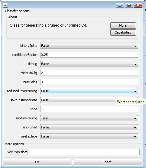
I used the default configuration parameter for J48 classifier. Here is the configuration menu.
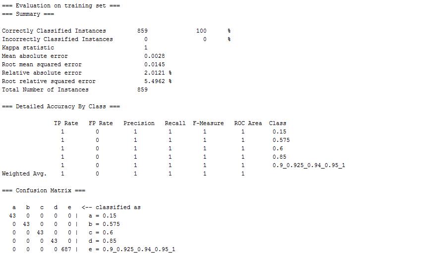
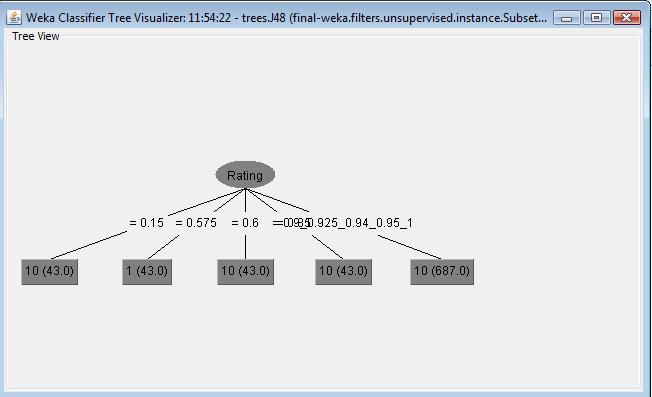
In first J48 classifier, I selected rating attribute as the target class lable. It builds a decision tree shown as the following. The evaluation part shows that all the data points are correctly classified and the error is minimized to 0 with Kappa statistic metric. Compared with Decision tree algorithm and Naive Bayes classifier with rating as the target class object, J48 is more suitable to analyze the data set and presents more accurate result. More text detail can be viewed here.
In second J48 classifier, I selected prize attribute as the target class lable. It builds a decision tree shown as the following. The evaluation part shows that all the data points are correctly classified. Also the classification error is 0 when using prize attribute as target class object. From the decision tree, we can observe certain relationship between rating value of prize value. Most records have high prize value 10 and the rating value varies from 0.15 to 1. The records that have low prize value 1 shows a relative low rating value 0.575. More text detail can be viewed here.
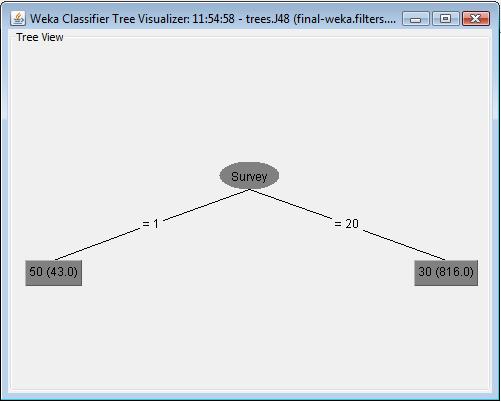
In third J48 classifier, I selected punishement attribute as the target class lable. It builds a decision tree shown as the following. The evaluation part shows that all the data points are correctly classified. Also the classification error is 0 when using punishement attribute as target class object. From the decision tree, we can observe certain relationship between survey value of punishment value. The group which have higher punishment value 50 have low survey value, while the group which have lower punishment value 30 have higher survey value. It might indicate that the reason why people has less score in survey is they receive high punishment in these ski resort. More text detail can be viewed here.
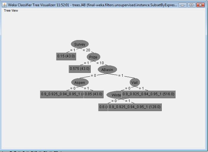
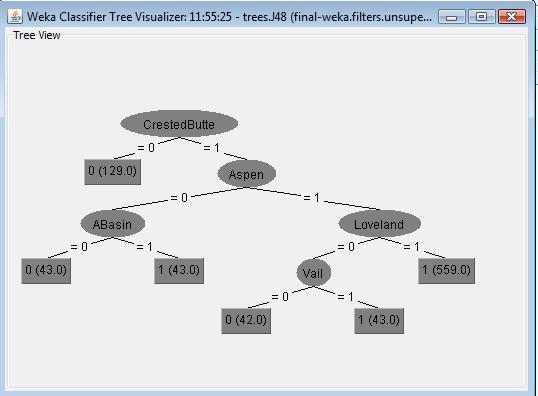
In forth J48 classifier, I selected one ski resort attribute snowmass as the target class lable. It builds a decision tree shown as the following. The evaluation part shows that all the data points are correctly classified. Also the classification error is 0 when using punishement attribute as target class object. From the decision tree, we can observe certain relationship among the set of ski resorts. For example, the group which selected snowmass ski resort tends to select crestedButte, aspen, Loveland ski resort as well. If they do not select crestedButte in the survey, they do not likely select snowmass either. We can infer that the similar correlation relationship among a suit of ski resorts might be observed when we choose other ski resort attribute as the target class object. More text detail can be viewed here.
Association Rule Mining
The association rule mining process is finding out the correlation relationship among the attribute sets. Followins is the workflow I created with Aprior algorithm in WEKA. The decretize part of the work flow is same as what I did in Naive Bayes classifer, because Aprior algorithm works with the nominal class object to discover the frequent item set. Next I used 4 aprior algorithm modules and applied each aprior algorithm in the selected attribute set. The WEKA project file is here.

I used remove filter to selecte the subset of attributes. Here is the configuration paramters for one of remove filters. This remove filter removed the first four attributes rating, survey, prize, punishment from the data set. After applying the remove filter, the dataset only contains the ski resort attributes so that the aprior algorithm can focus to discover the correlation relationship among different ski resorts. Using the remove filters with different paramters, I constructs the dataset with different attribute subset for mining association rules.

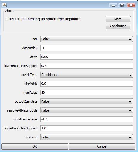
The aprior algorithm is one implementation of association rule mining algorithms. Here is the configuration parameter for the aprior algorithm. To find out more meaningful association rule, I set the minimum support as 0.7 and expands the number of rules to 50.
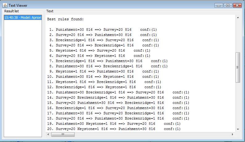
In first aprior algorithm module, I linked the whole attribute sets for aprior association mining process. The discovered association rule is shown as the following. Several association rules are reversed. For example, Punishment=30 816 ==> Survey=20 816, while the opposite rule Survey=20 816 ==> Punishment=30 holds as well. We might infer from these two rule that if people receive less punishement, they would like to give high score in survey. Combining other discovered rules, we can also get some interesting conclusion. With rule Breckenridge=1 816 ==> Punishment=30 and Keystone=1 816 ==> Punishment=30, it might indicate that people who select Breckenridge and Keystone receive less punishment. More text detail can be viewed here.
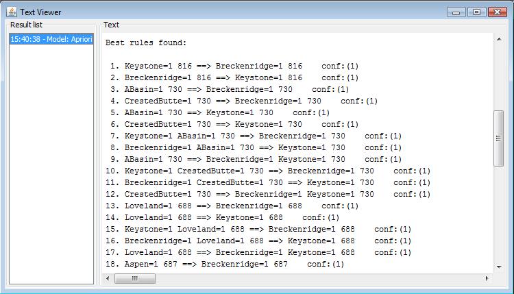
In the branch of second aprior algorithm module, I constructed the dataset with subset attribute sets. The aprior algorithm only deals with the ski resort attributes for mining process. The discovered association rule is shown as the following. It reveals that certain association relationship exists in different ski resorts. From the rules: Snowmass=1 Keystone=1 CrestedButte=1 645 ==> Breckenridge=1, Snowmass=1 Breckenridge=1 CrestedButte=1 645 ==> Keystone=1, Snowmass=1 Breckenridge=1 Keystone=1 645 ==> CrestedButte=1, Snowmass=1 CrestedButte=1 645 ==> Breckenridge=1 Keystone=1. We can inter that the four ski resorts, Snowmass, Keystone, CrestedButte, Breckenridge might have certain similarity or their location is close so that people tend to select the four ski resorts together. More text detail can be viewed here.
In the branch of third aprior algorithm module, I only include first 4 attributes of the dataset: rating, survey, prize and punishement. The aprior algorithm only deals with these four attributes to discover whether there is pattern to impact the rating value. The discovered association rule is shown as the following. Besides the same rules that has been discovered in the first aprior module, I also looked at the rules about the rating value. From the rules: Rating=0.9_0.925_0.94_0.95_1 687 ==> Survey=20, Rating=0.9_0.925_0.94_0.95_1 687 ==> Prize=10, Rating=0.9_0.925_0.94_0.95_1 687 ==> Punishment=30, we can infer that people who give the high rating also scores high in survey, receive more prize and less punishment. More text detail can be viewed here.

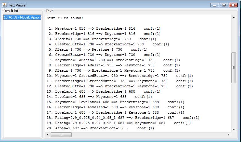
In the branch of forth aprior algorithm module, I include rating attribute and all the ski resort attributes of the dataset. The aprior algorithm aims to discover the relationship between the selection of ski resorts and rating value. The discovered association rule is shown as the following. From the rule: Rating=0.9_0.925_0.94_0.95_1 687 ==> Breckenridge=1, Rating=0.9_0.925_0.94_0.95_1 687 ==> Keystone=1, we might image that people who have high rating value tends to select Breckenridge and Rating ski resort. More text detail can be viewed here.
Conclusion
Pre-processing a first step in mining process of the data set. In pre-processing stage, I checked the missing value, identified the noise data, and also transformed the attribute value into the proper type for the following mining process. All these processes are very helpful to produce a valid data set and improve the accuracy of the mining strategies. Whiling considering the possible options to deal with missing and unclear values, I found that the confused records all have the identical values in all attributes via the visualization tool. These records are highly possible introduced due to certain error thus I decided to delete all these records containing missing or unclear columns. To save the result from pre-processing, I saved the processed dataset into a new data file so that the processed data set can be directly imported in the following mining processes.
I used four types of mining strageties and each strategy shows certain pattern from different point of view. Observing the clusters constructed by SimpyKmeans algorithm, the group with rating 0.15 have clear features: they have low score in survey, low value in prize and receive high punishment, and do not select any of ski resort. In classification analysis, the group labeled high rating value have high score in survey, high value in prize, receive less punishment and would like to select ski resort with different combinations. The association rules tends to mining the correlation relationship among attributes sets. I run the aprior algorithm in different attribute subsets and couple of miningful relationship has been discovered in the data set, as described in the previous section.
The mining process applied different strategies also shows the comparison result from different techniques. I used naive Bayes classifier and decision tree classifer to derive the classification model from the data set. The given class type in mining process is rating value and the discretize strategy is same in two classifiers. Though both classifers reach high accurate classification model and reveals the similiar pattern in the classification group, the evaluation metric indicates decision tree gives a model with error as 0, while model derived from naive bayes classifiers has error as 5.5%. From the point view of accuracy, we know decision tree algorithm is more suitable in the given dataset.