Bayesian Classifiers

Introduction

Bayesian Classifiers are typicially applied in the applications where the relationship between the attribute set and the class variable is non-deterministic. In other words, the class label of a test record can not be predicted with certainty even though its attribute set is identical to some of the training examples. It uses Bayes theorem, a statistical theorem for combining prior knowledge of the classes with new evidence gathered from data, to model probabilistic relationshios between the attribures and the class variables.

Bayes Theorem

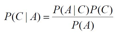
Bayes theorem shows the relation between two conditional probabilities which are the reverse of each other. A conditional probability is the probability that a random variable will take on a particular value given that the outcome for another random variable is known. It expresses the conditional probability of C given A, i.e., P(C|A), in terms of a reversed conditional probability of A given C, i.e., P(A|C). The formal equation of Bayes Theorem is shown [ 1 ] :

Bayesian Classifier

Bayes Classifiers created a probabilistic framework for solving classification problems. It considers the attribute set A and the class label C as random variables and capture their relationship probabilistically using P(C|A). The goal of bayes classifiers is to predict most accurate class C. Specifically, the class value C will be found by maximizing the conditional probability P(C|A). P(C|A) refers to the probability that the test record will be classified as class C given the oberserved data attributes A. This conditional probability is also known as the posterior probability for C, as opposed to its prior probability, P(C).

However, estimating the posterior probabilities P(C|A) accurately for every possible combination of class label and attribute value is a difficult problem because it requires a very large training set, even for a moderate number of attributes. The Bayes theorem describes an approach to compute the posterior probability P(C|A) in terms of the prior probability P(A), that is P(C|A)=P(A|C) x P(C)÷P(A). Choosing the value of C that maximize P(C|A) is equal to choosing the value of C that maximize P(A|C) x P(C) because the denominator term P(A) is always constant and can be ignored. The prior probability P(C) can be computed from the training set by computing the fraction of training records that belong to each class.

Different assumptions and methods are made in various Bayesian Classifiers. Naive Bayes classifiers assumes the attributes are conditionally independent and introduces a practical approach to computes the class-conditional probabilities P(A|C). Bayesian Belief networks adopts a flexible approach to model tthe class-conditional probabilities P(A|C). It allows us to specify which pair of attributes are conditionally independent instead of requiring all the attributes to be conditionally independeent given the class in Naive Bayes classifiers. A bayesian belief network creats a network structure to represent the probabilistic relationship among a set of attribute variables. Once the right topology has been found, the probability associated with each attribute is determined by using the similar approach in Naive Bayes classifiers.

Naive Bayes Classifier

A Naive Bayes classifier estimates the class-conditional probability by assuming that the attributes are conditionally independent, given the class lable C. The conditional indenpendence assumption can be formly stated as follows [ 1 ] :

where each attribute set A={A₁, A₂, ..., A_n} consists of n attributes.

With the conditional independence asumption, we can estimate the conditional probability P(A|C) by computing P(A_i|C_j) for each A_i, given C_j. Compared with directly computing P(A|C) in a large data set, this is a more practical approach because it does not require a very large training set to obtain a good estimate of the probability.

Two approaches are applied to estimate the conditional probabilites P(A_i|C_j) for categorical and continuous attributes.

• Estimating Conditional Probabilities for Categorical Attributes: It is straight forward to estimate conditional probabilities for a categorical attribute A_i. It is computed according to the fraction of training instances in class C_j that take on a particular attribute value A_i.
• Estimating Conditional Probabilities for Continuous Attributes: There are two ways to estimate the class-conditional probabilities for continuous attributes in Naive Bayes classifiers.
  • Discretize each continuous attributes

    It transforms the continuous attributes into ordinal attributes and then estimates the conditional probability P(A_i|C_j) by computing the fraction of training records belonging to class C_j that falls within the corresponding interval for the particular attribute value A_i. In this method, one can expect that the estimation error depends on the discretization strategy, as well as the number of discrete intervals. If the number of interval is too large, there are two few training records in each interval to provide a reliable estimation. On the other hand, if the number of intervals is too small, then some intervals may aggregate records from different classes and we may miss the correct dicision boundary.

  • Probability Density Estimation

    It assumes that the attribute sets follows a certian form of probability distribution and estimates the parameters of the distribution function using the training data set. For example, a Gaussian distribution is usually chosen to represent the probability distribution of random variables. The Gaussian distribution is characterized by two parameters, mean and standard deviation. Assum each attribute variable follows the Gaussian distribution, then the mean can be computed by the sample mean of A_i for all training data. Similarly, the standard deviation can be computed from the stardard deviation of same training data sets. Once the probability distribution is know, we can use it to estimate the conditional probabilities P(A_i|C_j).

Here is an example function [ 2 ] to implement the naive bayes classifier. It will calculate the probability for each category, and will determine which one is the largest and whether it exceeds the next largest by more than its threshold. If none of the categories can accomplish this, the method just returns the default values.

def classify(self,item,default=None):
probs={}
# Find the category with the highest probability
max=0.0
for cat in self.categories( ):
probs[cat]=self.prob(item,cat)
if probs[cat]>max:
max=probs[cat]
best=cat
# Make sure the probability exceeds threshold*next best
for cat in probs:
if cat==best: continue
if probs[cat]*self.getthreshold(best)>probs[best]: return default
return best

Conclusion

In general, Naive Bayes classifiers are robust to noise data because such noise data are averaged out when estimating the conditional probabilities from all data set. Naive Bayes classifiers are also practical classifiers to handle the irrelevant attributes. Using Bayes Theorem, it can get a good estimate of the probability and do not require a very large training set. However, if the attributes are correlated, the conditional independence assumption in Naive Bayes classifiers no longer holds. Bayesian Belife network is more flexible to model the conditional probability among correlated attribute sets. Bayesian Belife network provides an approach for capturing the prior knowledge of a particular domain using a graph model. The network model probabilistically combines with prior knowledge, it is also quite robust to model overfitting.

References

[1] Introduction to Data Mining, Pang-Ning Tan, Michael Steinbach, Vipin Kumar, Published by Addison Wesley.

[2] Programming Collective Intelligence, Toby Segaran, First Edition, Published by O’ Reilly Media, Inc.