Mining Similarity Using Euclidean Distance, Pearson Correlation,and Filtering
Similarity Measurement
Similarity metric is the basic measurement and used by a number of data ming algorithms. It measures the similarity or dissimilarity between two data objects which have one or multiple attributes. Informally, the similarity is a numerical measure of the degree to which the two objects are alike. It is usually non-negative and are often between 0 and 1, where 0 means no similarity, and 1 means complete similarity. [ 1 ]
Considering different data type with a number of attributes, it is important to use the appropriate similarity metric to well measure the proximity between two objects. For example, euclidean distance and correlation are useful for dense data such as time series or two-dimensional points. Jaccard and cosine similarity measures are useful for sparse data like documents, or binary data.
This page then contain a brief discussion of several important similarity metric.
Euclidean Distance
Euclidean Distance between two points is given by Minkowski distance metric. It can be used in one-, tow-, or higher-dimensional space. The formula of Euclidean distance is as following. [ 3 ]
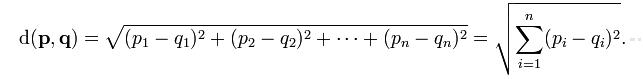
where n is the number of dimensions. It measures the numerial difference for each corresponding attributes of point p and point q. Then it combines the square of differencies in each dimension into an overal distance.
Here is an python example of calculating Euclidean distance of two data objects. This function calculates the distance for two person data object. It normalize the similarity score to a value between 0 and 1, where a value of 1 means that two people have identical preference, a value of 0 means that two people do not have common preference. [ 2 ]
from math import sqrt
# Returns a distance-based similarity score for person1 and person2
def sim_distance(prefs,person1,person2):
# Get the list of shared_items
si={}
for item in prefs[person1]:
if item in prefs[person2]:
si[item]=1
# if they have no ratings in common, return 0
if len(si)==0: return 0
# Add up the squares of all the differences
sum_of_squares=sum([pow(prefs[person1][item]-prefs[person2][item],2)
for item in prefs[person1] if item in prefs[person2]])
return 1/(1+sum_of_squares)
Pearson Correlation
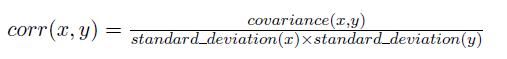
The correlation coefficient is a measure of how well two sets of data fit on a straight line. Correlation is always in the range -1 to 1. A correlation of 1 (-1) means that x and y have a perfect positive (negative) linear relationship. If the correlation is 0, then there is no linear relationship between the attributes of the two data objects. However, the two data objects might have non-linear relationships.
Pearson correlation is defined by the following equation. x and y represents two data objects.
Here is an python example of calculating Pearson Correlation of two data objects. The code for the Pearson correlation score first finds the items rated by both critics. It then calculates the sums and the sum of the squares of the ratings for the two critics, and calculates the sum of the products of their ratings. Finally, it uses these results to calculate the Pearson correlation coefficient, shown in bold in the code below. Unlike the distance metric, this formula is not very intuitive, but it does tell you how much the variables change together divided by the product of how much they vary individually. [ 2 ]
# Returns the Pearson correlation coefficient for p1 and p2
def sim_pearson(prefs,p1,p2):
# Get the list of mutually rated items
si={}
for item in prefs[p1]:
if item in prefs[p2]: si[item]=1
# Find the number of elements
n=len(si)
# if they are no ratings in common, return 0
if n==0: return 0
# Add up all the preferences
sum1=sum([prefs[p1][it] for it in si])
sum2=sum([prefs[p2][it] for it in si])
# Sum up the squares
sum1Sq=sum([pow(prefs[p1][it],2) for it in si])
sum2Sq=sum([pow(prefs[p2][it],2) for it in si])
# Sum up the products
pSum=sum([prefs[p1][it]*prefs[p2][it] for it in si])
# Calculate Pearson score
num=pSum-(sum1*sum2/n)
den=sqrt((sum1Sq-pow(sum1,2)/n)*(sum2Sq-pow(sum2,2)/n))
if den==0: return 0
r=num/den
return r
Jaccard Coefficient
Jaccard coefficient is often used to measure data objects consisting of asymmetric binary attributes. The asymmetric binary attributes have two values , 1 indicates present present and 0 indicates not present. Most of the attributes of the object will have the similiar value.
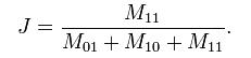
The Jaccard coefficient is given by the following equation:
where
M11 represents the total number of attributes where object A and object B both have a value of 1.
M01 represents the total number of attributes where the attribute of A is 0 and the attribute of B is 1.
M10 represents the total number of attributes where the attribute of A is 1 and the attribute of B is 0. [ 4 ]
Tanimoto Coefficient(Extended Jaccard Coefficient)
Tanimoto coefficient is also known as extended Jaccard coefficient. It can used for handling the similarity of document data in text mining. In the case of binary attributes, it reduces to the Jaccard coefficent. Tanimoto coefficent is defined by the following equation:
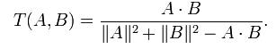
where A and B are two document vector object.
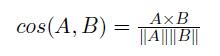
Cosine similarity
The cosine similarity is a measure of similarity of two non-binary vector. The typical example is the document vector, where each attribute represents the frequency with which a particular word occurs in the document. Similar to sparse market transaction data, each document vector is sparse since it has relatively few non-zero attributes. Therefore, the cosine similarity ignores 0-0 matches like the Jaccard measure. The cosine similarity is defined by the following equation:
References
[1] Introduction to Data Mining, Pang-Ning Tan, Michael Steinbach, Vipin Kumar, Published by Addison Wesley.
[2] Programming Collective Intelligence, Toby Segaran, First Edition, Published by O’ Reilly Media, Inc.
[3] http://en.wikipedia.org/wiki/Euclidean_distance
[4] http://en.wikipedia.org/wiki/Jaccard_index