Artificial Neural Network (ANN)

Introduction

Analogous to human brain structure, an ANN model is composed of an interconnected assembly of nodes and directed links. Neurologists have discovered that the Human brain learns by changing the strength of the synaptic connection between neurons upon repeated stimulation by the same impulse. Inspired by the biological neural system, the ANN model learns the training set by adjusting the weight parameters until the outputs of the perceptron become consistent with the true output of training examples.

Perceptron

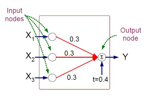
A simple neural network architecture is called perceptron. The perceptron consists of two types of nodes: input nodes, which are used to represent the input attributes, and an output node, which is used to represent the model output. In a perceptron, each input node is connected via a weighted link to the output node. The weighted link is used to emulate the strength of synaptic connection between neurons, which is input node and output node in perceptron model. As in biological neural systems, training a perceptron model amounts to adapting the weights of the links until they fit the input-output relationships of the underlying data.

The figure [ 1 ] shows an example perceptron architecture. It contains 3 input nodes (x1, x2, x3) and an output node y. Each input node has an identical weight of 0.3 to the output node and a bias factor of t = 0.4. The output node computes the weighted sum of the input value, subtracts the bias factor, and then produces an output that depends on the sign of the resulting sum. More specifically, the output of a perceptron model can be expressed mathematically as follows:

where wi are the weights of the input links and xi are the input attribute values. The sign function, which acts as an activation function for the output node, outputs a value +1 if its argument is positive and -1 if its argument is negative.

Learning Perceptron Model

The key computation for perceptron learning algorithm is finding out the best weight vectors applied in the model. The algorithm repeated updating the weight parameters in each iteration until the perceptron is consistent with the outputs of training dataset. The idea for adjusting weight is intuitive. The new weight is a combination of the original weight and a part based on the prediction error. If the prediction is correct, then the weight remains unchanged. Otherwise, it is modified.

In the weight update algorithm, links that contribute the most to the prediction error are the ones that require the largest adjustment. However, the amount of adjustment should be moderate. Otherwise, the adjustment we made in earlier iteration will be undone with drastical changes.The weight algorithm has a learning rate parameter λ to control the amount of adjustment made in each iteration. The value of λ is between 0 and 1. If λ is close to 0, then the new weight is mostly influenced by the value of the old weight. On the other hand, if λ is close to 1, then the new weight is sensitive to the amount of adjustment performed in the current iteration.

The basic operation of perceptron learning algorithm is formally illustrated in the following sudo code. [ 1 ]

   
Algorithm: Perceptron learning algorithm.
Input: Let D={(xi,yi)|i=1,2,...,N} be the set of training examples.
step 1: initialize the weight vector with random values, w(0).
step 2: repeat
           for each tranning example (xi, yi) in set D, do
               compute the predicted output y(k)
	       for each weight w_j do
		 update the weight, w_j(k+1)=w_j(k)+ &lambda(yi-yi(k))xij
	       end for
	   end for
	until stopping condition is met. 	
   

Multilayer Artificial Neural Network

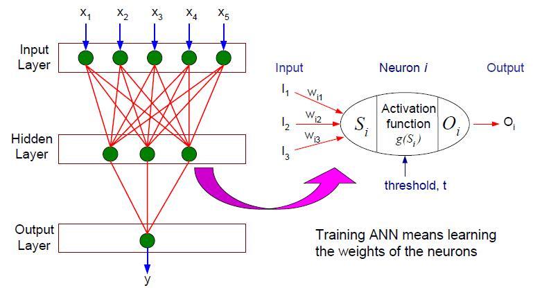
The multilayer artificial neural network contains several intermediary layers between its input and output layers. The intermediary layers are also called hidden layers and the nodes embedded in these layers are called hidden nodes. An example of feed-forward neural network architecture [ 1 ] is shown as below. The multilayer artificial neural network may use other types of activation functions other than the sign function, for example, linear function, sigmoid function, hyperbolic tangent functions and so an. These various type activation functions allow the hidden and output nodes to model non-linear relationship between the input parameters and output values.

The goal of the multilayer artificial neural network learning algorithm is to determine a set of weights w that minimize the total sum of squared errors:

In the error function [ 1 ] , the term f(Wi-Xi) states the predicted class which is a function of the weights assigned to the hidden and output nodes.

However, the global optimization is not trivial because it is difficult to determine the error term associated with each hidden node.A technique known as back-propagation has been developed to address this problem. It uses the errors for neurons at layer k+1 to estimate the errors for neurons at layer k. The basic computation of back-propagation can be breaken into two phases:

• forward phase: The computation progresses in the forward direction. Outputs of the neurons at level k are computed prior to computing the outputs at level k+1.
• backward phase: The computation progresses in the backward direction. the weights at level k+1 are updated before the weights at level k are updated.

Conclusion

The artificial neural network can be used to approximate any type of functions and relationships since one can define any network topology and use various type of activation functions. Considering its flexibility and large hypothesis space, it is important to choose the appropriate network topology for a given problem to avoid model overfitting. For example, the number of hidden layers, the hidden nodes, the type of activation function and feed-forward or recurrent network architecture must be determined before we train a neural network. Finding the right topology is not easy and might be very time consuming. The most appropriate topology is always determined depend on the problem and data set itself.

References

[1] Introduction to Data Mining, Pang-Ning Tan, Michael Steinbach, Vipin Kumar, Published by Addison Wesley.

[2] Programming Collective Intelligence, Toby Segaran, First Edition, Published by O’ Reilly Media, Inc.